added 10 characters in body
Source Link
user213
user213

It's not the gold standard, but you can sometimes get a good idea of the self noise of an instrument by looking at the distribution of noise values. Take a look at this image from the supplementary material of;

Ladegaard, M., Macaulay, J., Simon, M. et al. Soundscape and ambient noise levels of the Arctic waters around Greenland. Sci Rep 11, 23360 (2021). https://doi.org/10.1038/s41598-021-02255-6

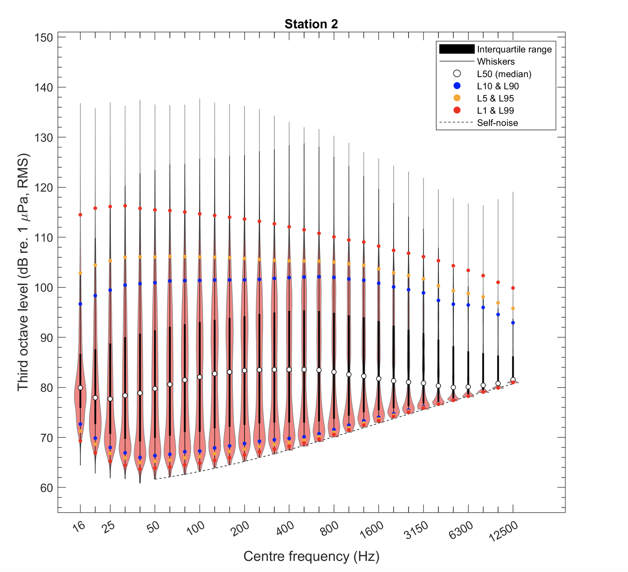
Violin plot of third octave noise levels. The thickness of each noise band measurement corresponds to the received distribution of noise levels. Coloured dots show the confidence intervals (see legend)

Long term noise measurements will usually form some sort of Gaussian like distribution - in this figure the noise values at lower frequency are higher amplitude and form the expected distribution. However, at higher frequencies the noise distributions begin to have a "hard edge" at the lower bound. This is almost certainly because the amplitude has fallen below the noise floor of the instrument (and so lower amplitude noise measurements are registered as the self noise of the instrument instead). Interpolating these lower bounds (dashed line) can provide an estimate of the noise floor of the instrument.
It's not the gold standard, but you can get a good idea of the self noise of an instrument by looking at the distribution of noise values. Take a look at this image from the supplementary material of;

Ladegaard, M., Macaulay, J., Simon, M. et al. Soundscape and ambient noise levels of the Arctic waters around Greenland. Sci Rep 11, 23360 (2021). https://doi.org/10.1038/s41598-021-02255-6

Violin plot of third octave noise levels. The thickness of each noise band measurement corresponds to the received distribution of noise levels. Coloured dots show the confidence intervals (see legend)

Long term noise measurements will usually form some sort of Gaussian like distribution - in this figure the noise values at lower frequency are higher amplitude and form the expected distribution. However, at higher frequencies the noise distributions begin to have a "hard edge" at the lower bound. This is almost certainly because the amplitude has fallen below the noise floor of the instrument (and so lower amplitude noise measurements are registered as the self noise of the instrument instead). Interpolating these lower bounds (dashed line) can provide an estimate of the noise floor of the instrument.

It's not the gold standard, but you can sometimes get a good idea of the self noise of an instrument by looking at the distribution of noise values. Take a look at this image from the supplementary material of;

Ladegaard, M., Macaulay, J., Simon, M. et al. Soundscape and ambient noise levels of the Arctic waters around Greenland. Sci Rep 11, 23360 (2021). https://doi.org/10.1038/s41598-021-02255-6

Violin plot of third octave noise levels. The thickness of each noise band measurement corresponds to the received distribution of noise levels. Coloured dots show the confidence intervals (see legend)

Long term noise measurements will usually form some sort of Gaussian like distribution - in this figure the noise values at lower frequency are higher amplitude and form the expected distribution. However, at higher frequencies the noise distributions begin to have a "hard edge" at the lower bound. This is almost certainly because the amplitude has fallen below the noise floor of the instrument (and so lower amplitude noise measurements are registered as the self noise of the instrument instead). Interpolating these lower bounds (dashed line) can provide an estimate of the noise floor of the instrument.

Source Link
user213
user213

It's not the gold standard, but you can get a good idea of the self noise of an instrument by looking at the distribution of noise values. Take a look at this image from the supplementary material of;

Ladegaard, M., Macaulay, J., Simon, M. et al. Soundscape and ambient noise levels of the Arctic waters around Greenland. Sci Rep 11, 23360 (2021). https://doi.org/10.1038/s41598-021-02255-6

Violin plot of third octave noise levels. The thickness of each noise band measurement corresponds to the received distribution of noise levels. Coloured dots show the confidence intervals (see legend)

Long term noise measurements will usually form some sort of Gaussian like distribution - in this figure the noise values at lower frequency are higher amplitude and form the expected distribution. However, at higher frequencies the noise distributions begin to have a "hard edge" at the lower bound. This is almost certainly because the amplitude has fallen below the noise floor of the instrument (and so lower amplitude noise measurements are registered as the self noise of the instrument instead). Interpolating these lower bounds (dashed line) can provide an estimate of the noise floor of the instrument.