2
$\begingroup$

I'm in my very first year of master's course and bioacoustic studies. My topic is the temporal/spectral structure of Rain call in Treefrog, which is poorly investigated for its function worldwide. Currently, I use Raven pro software only.

<Parameters>

1. Spectral parameter: Bandwidth, Dominant frequency

2. Temporal parameter: Number of note per call, Note duration, Note interval, Note rise time/fall time, Note repetition rate, Number of note per note, Pulse duration, Pulse interval, Pulse repetition rate

*Also, my professor suggested figuring out the patterns of peak amplitude of pulses.

<Troubles>

But as the calls were evoked randomly(as far as I experienced), thus most of the recording were held exceeding 5 to 10 meters away from calling individuals. (I can't measure the SNR though.)

These are the examples of my calls. All of them (Han window, window size:512, All calls were recorded with Marantz PMD 660 recorder and Senheiser SE64 shotgun Microphone with sampling rate of 44.1khz/32bit)

A)Waveform and spectrogram of Call_001, With bandpass filter under 6khz and 1second scale in line. enter image description here

B)Selection spectrum of one note of Call_001, same setting as above. enter image description here

C)Waveform of one note of Call_001, with 0.09s scale in line. enter image description here
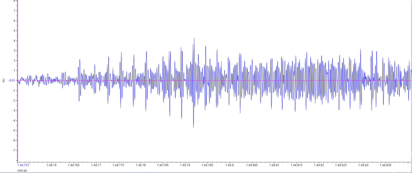
<Solution?>

How can I define the pulse duration in the note without a silent interval?

  1. I manually measure each pulse but this must lead to a bias.

  2. Then I try to use RMS amplitude as a threshold to define the end of each pulse. If so, the pulse peak under the RMS amplitude of each note will be defined as an end of a pulse.

If in this case, an increase of window length will be helpful to figure out temporal properties? Or if my calls are not enough to analyze under the time scale that much small?

<References>

These are my references, especially in terminology and ecological backgrounds.

1)Schad, K. (2007). Tree Calls Of Three Treefrogs (hyla Femoralis, H. Gratiosa, And H. Squirella): Analysis Of Environmental, Behavioral, And Acoustic Characteristics. <<<One and only research about rain call that i could reach.

2)Toledo, L. F., Martins, I. A., Bruschi, D. P., Passos, M. A., Alexandre, C., & Haddad, C. F. (2015). The anuran calling repertoire in the light of social context. Acta ethologica, 18, 87-99. <<< Brief, but meaningful summary of frog vocalization repertoire.

3)Koehler, J., Jansen, M., Rodriguez, A., Kok, P. J., Toledo, L. F., Emmrich, M., ... & Vences, M. (2017). The use of bioacoustics in anuran taxonomy: theory, terminology, methods and recommendations for best practice. Zootaxa, 4251(1), 1-124. <<< Most of my parameters were selected and defined by the terminology of this monograph.

Maybe my English and questions are elementary as I'm just a novice. But I hope you comment me any single idea or recommended articles to improve my study.

Sincerely.
$\endgroup$

2 Answers 2

3
$\begingroup$

If I understand correctly, you wanted to estimate inter alia the length of each note.

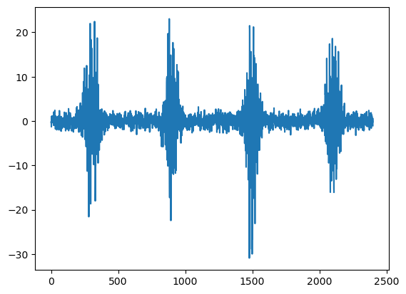
To demonstrate the algorithm I would start with, I wrote down two Python scripts that can be executed in a Jupyter notebook. The first simulates some data and generates a wav file, while the second script reads the wav file and carries out the processing.

import numpy as np
import matplotlib.pyplot as plt

# simulate pulse sequence
fs=1
ns=200
ss=np.random.randn(4,ns)*np.exp(-1/2*((np.arange(ns)-ns/2)/40)**2)
xx=np.random.randn(12*ns)
xx[int(1*ns):int(2*ns)]+=10*ss[0,:]
xx[int(4*ns):int(5*ns)]+=10*ss[1,:]
xx[int(7*ns):int(8*ns)]+=10*ss[2,:]
xx[int(10*ns):int(11*ns)]+=10*ss[3,:]
tx=np.arange(len(xx))/fs

plt.plot(tx,xx);
plt.show()

#---------------------------------------------------------
# store data as wav file
from scipy.io.wavfile import write

samplerate = fs;
write("example.wav", samplerate, xx.astype(np.int32))

Processing

import numpy as np
import matplotlib.pyplot as plt

# --------- load wav file ----------
from scipy.io.wavfile import read
fs,xx=read("example.wav")
tx=np.arange(len(xx))/fs

plt.plot(tx,xx);
plt.show()

# +++++++++++++++++++ processing+++++++++++++++++++++++++++
# accululate 'energy'
yy=np.cumsum(xx**2)
ty=np.arange(len(yy))/fs

# estimate sliding mean energy  
nw=10                               # ******can be better choice****
zz=(yy[nw:]-yy[:-nw])/nw
tz=(5+np.arange(len(zz)))/fs

# detect pulses
th=zz.std()                         # ******can be better choice****
id=np.where(zz>th)[0]

plt.plot(ty,yy)
plt.plot(tz,zz*100)
plt.plot(tz,th*100+0*tz)
plt.plot(tz[id],th*100+0*tz[id],'.')
plt.grid(True)
plt.show()

# min separation of notes
did=200  # samples                  # ******can be better choice****
spls=5+id[np.where(np.diff(id)>did)[0]]+did

# start stop indices of analysis widows
dets=np.vstack((np.append(0,spls),np.append(spls,len(yy))))
#print(dets.shape)
#print(dets)


idet=np.zeros((dets.shape[1],2),dtype=int)
for ii in range(dets.shape[1]):
    isel=range(dets[0,ii],dets[1,ii])
    i0=isel[0]
    uu=yy[isel]-yy[i0]
    uu = uu/uu[-1]
    plt.plot(ty[isel],uu)
    i1=np.where(uu>0.05)[0][0]      # ******can be better choice****
    i2=np.where(uu>0.95)[0][0]      # ******can be better choice****
    plt.plot(ty[i1+i0],uu[i1],'o')
    plt.plot(ty[i2+i0],uu[i2],'o')
    idet[ii,0]=i1+i0
    idet[ii,1]=i2+i0
plt.grid(True)
plt.show()

#print(idet)
# print note length
for ii in range(dets.shape[1]):
    print(ii,ty[idet[ii,1]]-ty[idet[ii,0]])

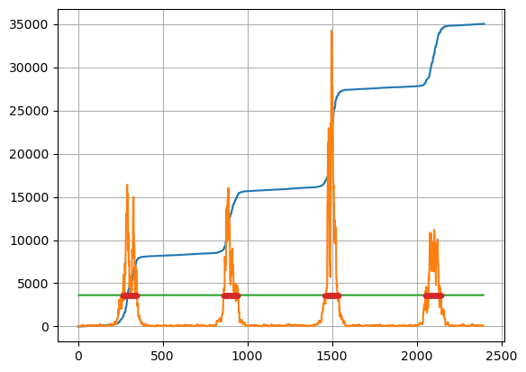
resulting in the following plots:

enter image description here

enter image description here

enter image description here

and finally the pulse length estimates

0 112.0
1 115.0
2 94.0
3 122.0

Note: The basic idea of estimating the note length is that it contains 90% of the signal energy (5 to 95 percentile).

For this, the different notes must first be detected. A simple threshold detector is sufficient. The one implemented here is based on the smoothed sound energy, but other detectors are possible, as long as they can be used to segment the time series into individual chunks that contain the pulses. Depending on the SNR the percentiles may need to be changed, but inspecting the pictures, it seems clear where a note starts and where it ends.

Anyhow, the present script can be sufficient to play with different data, parameter setting, etc.

Obviously, once the different processing steps are understood, then one can investigate the different software libraries for similar functionality.

In case it is too difficult to find the equivalent functionality in packages, like Raven Pro, maybe consider dedicated processing.

Edit: The above algorithm addresses the notes in your call that are separated by silent periods, but after multiple re-readings I have some doubt if you were also or foremost interested in the fine structure of a note, that you call pulses. I edit my answer in that sense and will add a new answer concerning fine structure of a note.

$\endgroup$
1
  • $\begingroup$ Modified the answer to save and read wav files $\endgroup$
    – WMXZ
    Commented Dec 4, 2023 at 20:06
1
$\begingroup$

2nd answer:

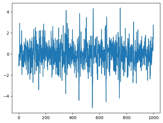
It seems that you also (foremost) wanted to estimate the fine structure of your note, which seems to be composed of multiple pulses.

once the individual notes are extracted from the time series, I see two estimates concerning the pulses:

  • inter-pulse-interval
  • pulse duration

The inter-pulse-interval (IPI) can be estimated using the autocorrelation. Here comes an example script

import numpy as np
import matplotlib.pyplot as plt
#
# simulate pulse sequence
fs=1
fo=0.1*fs
no=10       # number of pulses
nsp=100     # number of samples for pulse
nsn=no*nsp  # number od samples in note
ss=np.ones((no,1))*np.sin(2*np.pi*(np.arange(nsp)-nsp/2)*fo/fs)*np.exp(-1/2*((np.arange(nsp)-nsp/2)/(nsp/20))**2)
xx=np.random.randn(nsn)
for ii in range(ss.shape[0]):
    xx[int(ii*nsp):int(ii*nsp+nsp)] +=5*ss[ii,:]*np.exp(-1/2*((ii*nsp-nsn/2)/(nsn/4))**2)
plt.plot(xx)
plt.show()

# pulse interval estimation
# power autocorrelation
pc=np.fft.irfft(np.abs(np.fft.rfft(xx))**2)
plt.plot(pc)
plt.grid(True)
plt.show()
#
# print inper-pulse-interval
i1=1                    # minimal lag (could be half the expected interval in samples)
i2=int(len(pc)/2)       # limit to half of correlation lags
print(np.argmax(pc[i1:i2])/fs)

that generates the following output

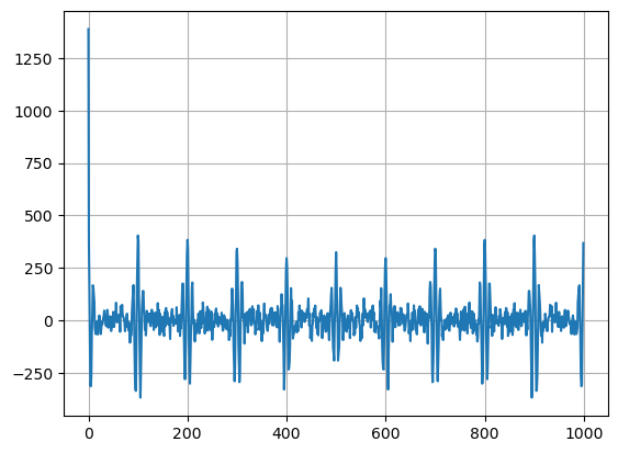
enter image description here enter image description here

99.0

The autocorrelation function is nothing than the inverse fft of the power spectrum of the signal. It has the dimension of time and describes the lages between the repetitive features (here pulses) in your signal (here note). BTW, this delay corresponds also to the spectral striping in your spectrogram, but this would be another answer.

Again, the script runs using Jupyter notebook and invites to play with the different parameters.

The second parameter you wanted to know is the length of the pulses. Now, this is extremely difficult without further restrictive assumptions. The observed pulses are overlapping, even if the transmitter (treefrog) will most likely emit the different pulse one after the other.

Obviously you can say, that the pulse length equals the IPI indicating that pulses are emitted without pauses. This would be the longest value.

If however the pulses emitted by the Treefrog are much shorter than the IPI value, then the fact that you do not see silence between pulses indicate that the environment corrupts your signal significantly to not allow realistic pulse-length estimation.

The autocorrelation function gives some indication on the pulse length (at least for simulated or reasonable clean data) and it is fair to say that the width of the autocorrelation function is for low time-bandwidth products about the width of the signal. For high time bandwidth products, the width of the peak in the autocorrelation function is reduced (keyword: pulse compression)

The width of the second peak in the cepstrum plot is about 30 time units which corresponds to about the simulated pulse width, if one considers $nsp/20 = \sigma = 5$ and gaussian pulse width being $2 \times 3\sigma$

Caveat: As usual, signal processing works alway fine in theory and with simulated data, but realty is full of surprises and pitfalls.

Edit: original answer contained the word Cepstrum, which was not correct. Cepstrum is the inverse Fourier Transform of the logarithm of the power spectrum. The presented script does not use the logarithm, so I changed the wordings. For this type of power spectrum, it turns out using the logarithm is not helping.

$\endgroup$
4
  • $\begingroup$ I'm very thankful to your comments, but I can hardly understand the codes. How can I load the recording file? $\endgroup$
    – Park
    Commented Dec 1, 2023 at 9:18
  • $\begingroup$ If you provide access to a wav file (say with 6 complete notes) I can improve my answers. $\endgroup$
    – WMXZ
    Commented Dec 1, 2023 at 16:27
  • $\begingroup$ Park, should we assume you've successfully setup Python and can run Jupyter notebooks? @WMXZ, without access to the files, you could still illustrate file access in python by restructuring your code into two parts: 1) create and write your signals to a wav file; 2) load the wav file and run your analyses. $\endgroup$
    – Brian Miller
    Commented Dec 4, 2023 at 3:27
  • $\begingroup$ @Brian, modified first answer to show possible use (read) of wav files $\endgroup$
    – WMXZ
    Commented Dec 4, 2023 at 20:07

Your Answer

By clicking “Post Your Answer”, you agree to our terms of service and acknowledge you have read our privacy policy.

Not the answer you're looking for? Browse other questions tagged or ask your own question.